Logistic Regression
Logistic regression predicts the probability of an outcome that can only have two values. Let’s take a data that having two classes, class -1 and class 1 as shown in below fig.
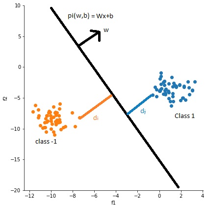
from above fig logiction regression function is to find the plane \(\pi (W,b)\) that best seperated the positive and negative classes. from above fig distance from point \(x_i\) to plane \(\pi\) i.e \(d_i\) = \(\frac{W^T.x_i+b}{||W||}\) and W is unit vector so ||W|| = 1.
so \(d_i > 0\) for all positive samples because w is in same direction and \(d_i < 0\) for all negative samples. if \(y_i = 1\) for positive points and -1 for negetive points. let’s assume plane is passing through origin i.e no intercept so b = 0. for correctly classified points \(y_iW^Tx_i > 0\) and for all wrong classified points \(y_iW^Tx_i < 0\). Main objective of classification is to classify correctly so out objective in Logistic regression is to find the W and b such that \(\sum_{i=1}^n (y_iW^Tx_i)\) is maximum.
So optimization problem is \[ W^* = argmax \sum_{i=1}^n (y_iW^Tx_i)\]
But this will fails in some conditions one of them is listed below.
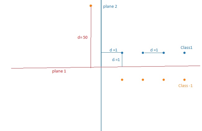
From above diagram for \(\pi_1\), \( \sum_{i=1}^n (y_iW_1^Tx_i)\) = 1+1+1+1+1+1+1+1-50 = -42 and for \(\pi_2\), \( \sum_{i=1}^n (y_iW_2^Tx_i)\) = 1+2+3+4-1-2-3-4+1 = 1. so plane \(\pi_2\) is better for maximizing the sum but we can see that accuracy of \(\pi_1\) is higher than \(\pi_2\). it is because of single outlier in our train data. we can overcome this by squeezing the maximum distance points into min distance. this can be done by sigmoid function as shown below.
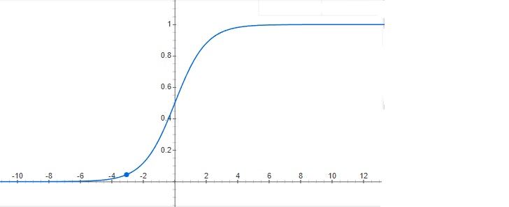
sigmoid function wil give values between [0,1] based on input real value. so we can decrese the outlier effect on the optimization problem.
so our optimization problem is \[ W^* = argmax \sum_{i=1}^n \sigma(y_iW^Tx_i)\]
from operations that preserve Argmax, if g(x) is monotonic function then argmax f(x) = argmax g(f(x)). if we take g(x) as a log fuction then we can get some good properties as converting exponent as mutiplication, converting multiplication into addition. so our final optimization problem is \[W^* = argmax \sum_{i=1}^n \log(\sigma(y_iW^Tx_i)) \]
\[W^* = argmax \sum_{i=1}^n \log(\frac{1}{1+e^{-y_iW^Tx_i}}) \]
\[W^* = - argmax \sum_{i=1}^n \log(1+e^{-y_iW^Tx_i}) \]
\[W^* = argmin \sum_{i=1}^n \log(1+e^{-y_iW^Tx_i}) \]
For regularization
\[L2 - W^* = argmin \sum_{i=1}^n \log(1+e^{-y_iW^Tx_i}) + \lambda ||W|| \]
\[L1 - W^* = argmin \sum_{i=1}^n \log(1+e^{-y_iW^Tx_i}) + \lambda |W| \]
after optimization we can predict by using \(W^Tx+b\)
Feature importance and Model interpretability:
if all features are almost independent then our Weight vetors W will give the how much is the effect of feature according to the feature weight. so if absolute value of feature weight is large then the feature is more important to predict the class. so for this all features must be independent so before getting feature importance have to check for independance i.e multicollinearity.
We can check multicollinearity by using perturbation test. for this testing add some value \(\delta\) to the data and agian recompute the weights lets name it as \(W_p\). campre W and \(W_p\) if any high changes in \(W_p\) then weight vector is not good choice to interpret the feature importance.
Time and Space complexity:
n = no of data instances, d = dimension of data
Train time complexity is nearly O(nd)
Rum time complexity is nearly O(d) because we have calculate only \(W^Tx_q\)
Run time space complexity is O(d) because need to save only weight vector
We can decrease the no of multiplication while prediction time by incresing the l1 regularization, because l1 regularization will increse the sparsity of Weight vector.
Here you can see total notebook that explains how to do hyperparameter tuning to Logistic Regression.
References:
- Applied AI Course
- https://en.wikipedia.org/wiki/Logistic_regression