Optimization

Optimization is a methodology for finding the maximum or minimum value of a real function.More generally,optimization includes finding “best available” values of some objective function given a defined domain (or input), including a variety of different types of objective functions and different types of domains.

Unconstrained Optimization:

In an unconstrained optimization problem, the task is to locate the solution x* that maximizes or minimizes f(x) without imposing anycconstraints on x. The solution x, which is known as a stationary point, can be found by taking the first derivative of f(x) and setting it to zero.

analytical method:

for analytical steps are given below:

Find the f’(x) and set it to zero and then find x = x*
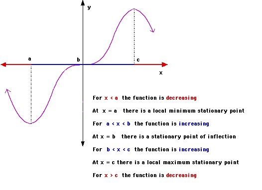
if f’‘(x) > 0 then x* is local minimum
if f’‘(x) < 0 then x* is local maximum
If f’‘(x) = 0 then x* is inflection point of f(x) as shown in below fig

maximum and Minimum
eg: \[f(x) = x^3 − 3x^2 − 45x \] \[f’(x) = 3^2 - 6x - 45 = 0 \] \[x^* = -3 \text{ or } x^* = 5\] \[f’‘(x) = 6x − 6\]
When x = -3, f ‘’(-3) = -24 and this means a MAXIMUM point.
When x = 5, f ‘‘(x) = 24 and this means a MINIMUM pont.
This definition can be extended to a multivariate function\(f(x_1,x_2…x_n)\),where the condition for finding a stationary point is \[\frac{\partial f}{\partial x_i} = 0 \text{ for all } x_1,x_2..x_n\] unlike univariate functions, it is more difficult to determine whether X* corresponds to a maximum or minimum stationary point.The difficulty arises because we need to consider the partial derivatives \(\frac{\partial^2 f}{\partial x_i \partial x_j}\) for all possible pairs of i,j. so this complete set is given by hessian matrix H(x).

X is minimum if H(x) is positive definite i.e \(X^THX > 0\) for any non-zero column vector X.
X is maximum if H(x) is negative definite i.e \(X^THX < 0\) for every non zero column vector X.
X is saddle point if H(x) is indefinite i.e for some values of X \(X^THX > 0\) and for some values \(X^THX < 0\)

eg: \[f(x,y) = 3x^2+2y^3-2xy\] \[\frac{\partial f}{\partial x} = 6x-2y = 0 \text{ and } \frac{\partial f}{\partial y} = 6y^2-2x = 0\] solution for above equation is \(x^* = y^* = 0 \text{ and } x^* = 1/27, y^* = 1/9\)
Hessain of f is\[ H(x,y) = \begin{bmatrix} 6 & -2 \newline -2 & 12y \end{bmatrix} \] For \(x^* = y^* = 0 \text{ value of }X^TH(0,0)X = 6x^2-4xy\) and this can be either positive or negative so at (0,0) Hessian is indefinite so (0,0) is saddle point.
For \(x^* = 1/27, y^* = 1/9 \text{ value of }X^TH(1/27,1/9)X = 4x^2-2xy+4y^2/3 = 4(x-y/4)^2+13y^2/4\) tis value is always >0 for non zero values of x,y. so te Hessian is a positive definite. Therefore, (1/27,1/9) is a minimum stationary point and minimum value is -0.0014.

Gradient Descent Method:

Gradient descent is a first-order iterative optimization algorithm for finding the minimum of a function.The gradient descent method assumes that the function f(x) is differentiable and computes the stationary point as follows \[x_0 = x_0 - \lambda \nabla(f)\] In this method, the location of x is updated in the direction of the steepest descent, which means that x is moved towards the decreasing value of f(x).

Newton’s Method:

Newton’s method is based on quadratic approximation to the function. By using a Taylor series expansion of f around \(x_0\) is \[ f(x) \approx f(x_0)+(x-x_0)f’(x_0)+\frac{(x-x_0)^2}{2}f’‘(x_0)\] \[ f’(x) = f’(x_0)+(x-x_0)f’‘(x_0) = 0\] \[ x = x_0 - \frac{f’(x_0)}{f’‘(x_0)}\] above equation can be used to update r until it converges to the location of the minimum value.
For multivariate functions the above equaton is \[x = x_0 - H^{-1}\nabla(f)\]

Constrained Optimization:

constrained optimization is the process of optimizing an objective function with respect to some variables in the presence of constraints on those variables. Constraints can be either hard constraints, which set conditions for the variables that are required to be satisfied, or soft constraints, which have some variable values that are penalized in the objective function if, and based on the extent that, the conditions on the variables are not satisfied.
a general constrained minimization problem may be written as follows \[ \text{Min} f(x) \text{ subject to }g_i(x) = c_i\text{ for i = 1,2,..n }h_j(x)\ge d_j \text{ for j = 1,2,..n }\]

Equality Constraints:

consider a a problem of finding the minimum value of \(f(x_1,x_2,x_3..x_n)\) subjected to equality constraints of form \(g_i(x) = 0\) for 1 = 1,2,3…d.
By using Lagrange multipliers above problem can be solved and steps are given below.

define the Lagrangian, \(L(x,\lambda) = f(x) + \sum_{i=0}^d \lambda_ig_i(x)\) where \(\lambda_i\) is called Lagrange multiplier.
compute \(\frac{\partial L}{\partial x_i} \text{ for i = 1,2,..n and } \frac{\partial L}{\partial \lambda_i} \text{ for i =1,2..d }\) and set it to zero. \[\frac{\partial L}{\partial x_i} = 0 \text{ for i = 1,2,..n }\] \[\frac{\partial L}{\partial \lambda_i} = 0 \text{ for i =1,2..d }\]
solve above eqations in step2 to obtain \(x^* \) and corresponding \(\lambda_i’s\)

eg: Minimize the f(x,y) = x + 2y subjected to constrint \(x^2+y^2-4=0\).
\[L(x,y,\lambda) = x+2y+\lambda(x^2+y^2-4)\] \[\frac{\partial L}{\partial x} = 1+2\lambda x = 0\] \[\frac{\partial L}{\partial y} = 2+2\lambda y = 0\] \[\frac{\partial L}{\partial \lambda} = x^2+y^2-4 = 0\] solving these eqations gives \(\lambda = \pm 5/4, x = \mp2/\sqrt{5}, y = \mp 4/\sqrt{5} \) so \(f(-2/\sqrt{5},-4/\sqrt{5}) = -10/sqrt{5},(f(2/\sqrt{5},4/\sqrt{5}) = 10/sqrt{5}\). so f(x,y) has minimum value at \(x = -2/\sqrt{5},y = -4/\sqrt{5}\).

Inequality Constraints:

consider a a problem of finding the minimum value of \(f(x_1,x_2,x_3..x_n)\) subjected to equality constraints of form \(h_i(x) \le 0\) for 1 = 1,2,3…d.
The method for solving this problem is quite similar to the Lagrange method described above. However, the inequality constraints impose additional conditions to the optimization problem. Lagrangian is \(L(x,\lambda) = f(x) + \sum_{i=0}^d \lambda_ih_i(x)\) and constraints known as KKT conditions \[\frac{\partial L}{\partial x_i} = 0 \text{ for i = 1,2,..n }\] \[h_i(x) \le 0 , \text{ for i = 1,2,3,..d }\] \[\lambda_i \ge 0 , \text{ for i = 1,2,3,..d }\] \[\lambda_ih_i(x) = 0 , \text{ for i = 1,2,3,..d }\]
Notice that the Lagrange multipliers are no longer unbounded in the presence of inequality constraints.
Eg: Minimize \(f(x,y) = (x-1)^2 + (y-3)^2\) subjected to x+y<=2 and y>=x.
Lagrangian is \[ L(x,y,\lambda_1,lambda_2) = (x-1)^2 + (y-3)^2 + \lambda_1(x+y-2) + \lambda_2(x-y)\] and KKT conditions are \[\frac{\partial L}{\partial x} = 2(x-1)+\lambda_1+\lambda_2 = 0\] \[\frac{\partial L}{\partial y} = 2(y-3)+\lambda_1-\lambda_2 = 0\] \[\lambda_1(x+y-2) = 0\] \[\lambda_2(x-y) = 0\] \[\lambda_1 \ge 0 , \lambda_2 \ge 0 , x+y \le 2, y \ge x\] So we have to solve above equations to get te solution for min values.

References: 1.Picture of Maxima and minima and example taken from http://bestmaths.net/online/index.php/year-levels/year-12/year-12-topic-list/stationary-and-turning-points/ 2.Applied AI Course 3.Introduction to data mining by Tan