Principal component analysis
PCA :
The goal of PCA is to find new set of dimensions that better captures the varibility of data. i.e. the first dimention is chosen to capture as much of varibility as posiible, second dimension is orthogonal to first and captures as much of remaining varibility as possible and so on.
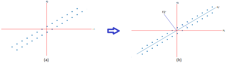
Lets assume we have two dimension data i.e (n x 2) matrix and if we want only one dimension,then i will only keep the data which is having more spread/varinace so my final data will be (n x 1) matrix which contains column which having more spread. but in some cases as below fig(a) we have spread on F1 and F2 both are high and if we drop any one dimention then we may loose data by very much. in that case, we can also see that in F1’ direction we have maximum spread and perpendicular to this is F2’ (fig(b)), so instaed of dropping F1 or F2, if we find F1’ and F2’ then we will get more spread in F1’ direction than F2’. after that we can drop F2’ and project points onto F1’. This is nothing but a rotation of axis F1 to some angle. so our aim is we want to find direction of F1’ such that variance of points projects onto F1’ is maximum.
Finding F1’:
Lets take any point from above diagram and call it as the \( x_i \) and projection onto F1’ is
\[ x_i’ = \frac{F_1’.x_i}{||F_1’||^2} \].
we need only direction of F1’ so F1’ is taken as unit vector and \( ||F_1’||^2\)= 1. i.e \( x_i’ \) = \( F_1’^T.x_i \).
so we have to increase the variance of \( F_1’^T.x_i \) for all values if i.
\[Var( F_1’^T.x_i ) = \frac{1}{n} \sum_{i=0}^n ({F_1’^T.x_i - F_1’^T.\bar x_i})^2\].
if data is standadized then \( \bar x_i \) = 0 so second term in variance = 0 so
\[ \sigma ^2 = \frac{1}{n} \sum_{i=0}^n ({F_1’^T.x_i})^2\].
so our opimization problem is have to find F1’ that maximizes variance such that \( F_1’ \) is unit vector. so optmization is
\[ Max \frac{1}{n} \sum_{i=0}^n ({F_1’^T.x_i})^2 s.t F_1’^T.F_1 = 1.\]
and covariance matrix S = \( \frac{1}{n} \sum_{i=1}^n x_i.x_i^T = \frac{X^T.X}{n} \) so we can change the above variance as \( F_1’^TSF_1\).We can solve this by Constrained optimization using lagrange multiplier and after changing to lagrange form
\[L(F_1’,\lambda ) = F_1’^TSF_1’ - \lambda(F_1’^TF_1’ - 1)\]
\[ \frac{\partial L}{\partial F_1’}= SF_1’ - \lambda F_1’ = 0 \]
\[ SF_1’ = \lambda F_1’\]
This is the definition of eigan vector where \(F_1’\) is eigan vector and \(\lambda\) is eigan value of S i.e covariance matrix of \(x_i\)’s.
Selecting the no of dimentions such that maxumum variance captured is one of main things while performing PCA to the data. from the eigan values and vectors we got \(\lambda_1,\lambda_2…\lambda_d\) and corresponding vectors\(F_1’,F_2’…,F_d’\). from this variance ratio of n dimensons is given by
\[ VarianceRatio = \frac{\lambda_1+\lambda_2+..+\lambda_d}{\sum_{i=1}^d(\lambda_i)}\]
variance ratio is in between 0 and 1 so we need to select n such that variance ratio is maximum or beased on ow much variace we need in our data.
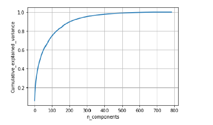
Above is the Gramph for cumulative variance ratio vs no of dimentions. from that we can observe that incresing the dimentions is increasing the variance ratio as well and around 500 dimensions is giving nearly 1 as ratio. We can also use PCA for data visualization in lower dimentions.
References:
- applied ai course
- https://en.wikipedia.org/wiki/Principal_component_analysis