Support Vector Machine
SVM is one type of classification and regression algorithm which is maily focused on the maximal margin hyperplane. Figure below shows two different classes seperating by three hyperplanes and also we can plot infinity hyperplanes to classify those two classes.
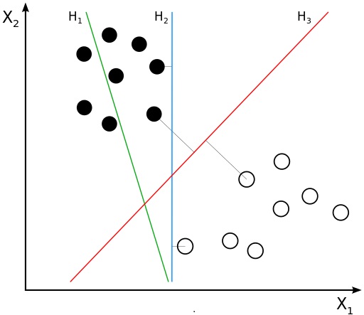
Although their training errors are zero for many of them, there is no guarantee that the hyperplanes will perform equally well on unseen data. The classifier must choose one of these hyperplanes to represent its decision boundary, based on how well they are expected to perform on test samples. Decision boundaries with large margins tend to have better generalization errors than those with small margins. Intuitively, if the margin is small, then any slight perturbations to the decision boundary can have quite a significant impact on its classification. Classifiers that produce decision boundaries with small margins are therefore more susceptible to model overfitting and tend to generalize poorly on previously unseen data, so SVM tries to locate the hyperplane such that distance is maximum from both the classes.
How SVM is selecting margin:
Consider a binary classification problem as shown in below figure and the hyperplane is \(\pi\). And two planes whcich are parallel to the hyperplane and passing through nearest point of each class are \(\pi_+\) and \(\pi_-\) as shown in below fig. and Those points are called as support vectors.
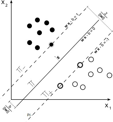
Maximizing margin means maximizing distance between the \(\pi_+\) and \(\pi_-\). So our objective is to maximize the distance between those two planes. Let’s assume for all positive points y = +1 and for all negative points y = -1 so \(y_i(W^Tx+b) \ge 1\) for all points. To compute the margin, let x1 be a data point located on \(\pi_+\) and x2 be a data point on \(\pi_-\).
\[\pi_+ is W^Tx_1 + b = +1\]
\[\pi_- is W^Tx_2 + b = -1\]
by subtracting
\[W.(x_1-x_2) = 2\]
\[||W|| * d = 2\]
\[d = \frac{2}{||W||}\]
so our optimization problem is
\[ Max \quad \frac{2}{||W||} \quad { S.T. } \quad y_i(W^Tx_i+b) \ge 1 \quad \forall \; i\]
Max x = Min 1/x so we can write our problem as
\[ \text{Min } \quad \frac{||W||}{2} \quad { S.T } \quad y_i(W^Tx_i+b) \ge 1 \quad \forall \; i\]
This SVM formulation presented in the previous section constructs only decision boundaries that are mistake-free. This is called Hard margin SVM. For non separable data all constraints wont satisfy. So The learning algorithm in SVM must consider the trade-off between
the width of the margin and the number of training errors committed by the decision boundary. For this introducing positive-valued slack variables \(\;\xi\;\) into the constraints of the optimization such that for all positive points in positive side \(\;\xi_i = 0\;\), for all negative points in negative side \(\;\xi_i = 0\;\), for all positive points in negative side \(\;\xi_i > 0\;\) and \(\;\xi_i\;\) is distance from \(\;\pi_+\;\), for all negative points in positive side (\;\xi_i > 0\;\) and \(\;\xi_i\;\) is distance from \(\;\pi_-\;\). \(\;\xi_i\;\) is high for the points far away from correct hyperplane \(\;\pi_+\;\) or \(\;\pi_-\).
So our new formulation is
\[( W^* , b^* ) = \text{ arg min }\; \frac{||W||}{2}+C(\frac{1}{n}\sum_{i=1}^n\xi_i) \quad { S.T }\quad y_i(W^Tx_i+b) \ge 1-\xi_i \; \forall i \; \text{ and } \; \xi_i > 0\]
We can observe that, above formulation can be assumed like \(\;C(\frac{1}{n}\sum_{i=1}^n\xi_i)\;\) as Loss and \(\;\frac{||W||}{2}\;\) as regularization term. \(\;\xi_i\;\) is the distance from correct hyperplane so \(\xi_i\) = 1 + absolute distance from decision hyperplane \(\pi\) for incorrectly classified points and 0 for correctly classified points. but As it turns out, distance alone is not as useful as distance inversely weighted by the margin size becuase distance is given by W^Tx_i+b/||W||. This can be explained by thinking of a specific example. Suppose a point is inside the margin by one unit. and it is worse when the margin is 2 units across than 200 units(margin width). When the margin is this small, penetrating it by even a small distance means the point is very close to being incorrectly classified. to remove this effect, we will remove ||W|| in denominator.
\[ \xi_i = \begin{cases}
1 \; + abs(W^Tx_i+b) \quad \text{ for incorrectly classified points } \newline
0 \quad \text{ for correctly classified points } \newline
\end{cases}\]
for incorrectly classified points the absolute distance can be written as \(-y_i(W^Tx_i+b)\), because \(W^Tx_i+b\) gives signed distance and and \(y_i\) is +1 for positive class and -1 for negative class. For positive class points in negative region \(W^Tx_i+b\) is negatative,\(y_i\) is positive so \(-y_i(W^Tx_i+b)\) is positive. for negative class points in positive region \(W^Tx_i+b\) is positive,\(y_i\) is negative so \(-y_i(W^Tx_i+b)\) is positive.
\[ \xi_i = \begin{cases}
1 \; - y_i(W^Tx_i+b) \quad \text{ for incorrectly classified points } \newline
0 \quad \text{ for correctly classified points } \newline
\end{cases}\]
also for correctly classified points \(-y_i(W^Tx_i+b)\) is negative so we can write as \[ \xi_i = MAX(0\;,1 \; - y_i(W^Tx_i+b))\] final optimization problem is \[ Min \; C(\sum_{i=1}^n \; MAX(0\;,1 \; - y_i(W^Tx_i+b))) \; + \; \frac{||W||}{2}\] This is nothing but a Hing Loss. Where C is the hyperparameter, if C increses ten frequency to make mistakes will be decresed,this may led to overfitting to data. If C decreses frequency to make mistakes increases, this may lead to underfit.If C=0, then this is hard margin SVM.
Solution for Optimization:
our optimization problem is to minimize \(\frac{||W||}{2}\) such that \(y_i(W^Tx_i+b) \ge 1 \; \forall i = 1,2..n\). so Lagrangian is (for optimization tutorial you can see here)
\[ L \;= \frac{||W||}{2} \; - \; \sum_{i=1}^n \alpha_i(y_i(W^Tx_i+b)-1)\]
KKT conditions are
\[ \frac{\partial L}{\partial W} \; = \; W - \sum_{i=1}^n \alpha_iy_ix_i = 0\]
\[\frac{\partial L}{\partial b} \; = \; -\sum_{i=1}^n\alpha_iy_i = 0\]
\[ \alpha_i \ge 0 \quad \text{ and } \alpha_i(y_i(W^Tx_i+b)-1) = 0 \]
so from above two eqations \( W = \sum_{i=1}^n \alpha_iy_ix_i\) and \(\sum_{i=1}^n \alpha_iy_i = 0\).
Subtituting these values in Lagrangian L
\[ L \;=\; \frac{1}{2}(\sum_{i=1}^n\alpha_iy_ix_i)(\sum_{i=1}^n\alpha_iy_ix_i) - \sum_{i=1}^n\alpha_iy_ix_i.W - \sum_{i=1}^n\alpha_iy_ib + \sum_{i=1}^n\alpha_i\]
\[ L \;=\; \frac{1}{2}(\sum_{i=1}^n\alpha_iy_ix_i)(\sum_{i=1}^n\alpha_iy_ix_i) - (\sum_{i=1}^n\alpha_iy_ix_i)(\sum_{i=1}^n\alpha_iy_ix_i) - \sum_{i=1}^n\alpha_iy_ib + \sum_{i=1}^n\alpha_i\]
\[ L \;=\; -\frac{1}{2}(\sum_{i=1}^n\alpha_iy_ix_i)(\sum_{i=1}^n\alpha_iy_ix_i) - \sum_{i=1}^n\alpha_iy_ib + \sum_{i=1}^n\alpha_i\]
\(\sum_{i=1}^n\alpha_iy_ib\) will be zero because b is constant and \(\sum_{i=1}^n \alpha_iy_i = 0\).
\[ L \;=\; \sum_{i=1}^n\alpha_i -\frac{1}{2}(\sum_{i=1}^n\alpha_iy_ix_i)(\sum_{j=1}^n\alpha_jy_jx_j)\]
\[ L \;=\; \sum_{i=1}^n\alpha_i -\frac{1}{2}(\sum_{i=1}^n\sum_{j=1}^n \alpha_i\alpha_jy_iy_jx_ix_j)\]
here conditions are \(\;\alpha_i \ge 0\;\) and \(\;\sum_{i=1}^n \alpha_iy_i = 0\;\). This is called as Dual formulation of SVM. This has many advantages over primal formulation.
After solving above dual formulation we will get \(\;\alpha_i\;\) > 0 for all support vectors and = 0 for others.For classifying a query point we will use \(\;W^Tx_q+b)\;\) sign i.e. \(\;\sum_{i=1}^n\alpha_iy_ix_ix_q+b\;\). With only support vectors we can classify our query point because for others \(\;\alpha_i = 0\).
How SVM works for non linear data:
The trick here is to transform the data from its original coordinate space in x into a new space \(\;\phi(x)\;\) so that a linear decision boundary can be used to separate the instances in the transformed space like below fig.
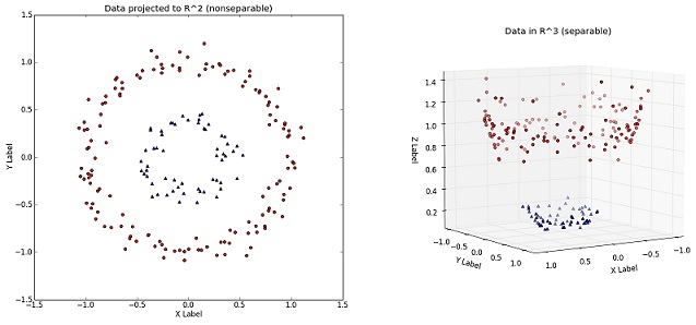
So a non linear transformation \(\;\phi\;\) needed to map the data from its original feature space into a new space where the decision boundary becomes linear. after transforming, solving the constrained optimization problem in the high-dimensional feature space is a computationally expensive task.We can observe from above dual formulation that \(\;x_i.x_j\;\) is the dot product between the features.The dot product is often regarded as a measure of similarity between two vectors. for eg. the cosine similarity can be defined as the dot product between two vectors that are normalized to unit length. so dot product between \(\;\phi(x_i) , \phi(x_j)\;\) can also be regarded as a measure of similarity between two instances, \(\;x_i,x_j\;\), in the transformed space. This similarity function is called as the kernal function. Kernel functions always expressed as the dot product between two input vectors in some high-dimensional space.
Polynomial kernal:
\[k(x,y)\; = \; (x.y+1)^d\] for d = 2 \[k(x,y)\; = \; (x.y+1)^2\] \[k(x,y)\; = \; (1+x_1y_1+x_2y_2)^2\] \[k(x,y)\; = \; (1+x_1^2y_1^2+x_2^2y_2^2+2x_1y_1+2x_2y_2+2x_1y_1x_2y_2)\] \[k(x,y)\; = \; (1,x_1^2,x_2^2,\sqrt2x_1,\sqrt2x_2,\sqrt2x_1x_2)^T.(1,y_1^2,y_2^2,\sqrt2y_1,\sqrt2y_2,\sqrt2y_1y_2)\] \[k(x,y)\; = \; \phi(x_i).\phi(x_j)\]
RBF kernal:
\[k(x,y)\; = \; e^{\frac{- ||x_1 - x_2||^2}{2\sigma^2}}\] Here \(- ||x_1 - x_2||^2\) may be recognized as the squared Euclidean distance between the two feature vectors. \(\;\sigma\;\) will give the width if that kernal. intuitively we are getting distance between points in a given range, similar to the KNN. Here \(\;\sigma\;\) is hyperparameter and free to optimize. \(\;\sigma\;\) is increasing means we are considering similarity of larger distance points also. so low \(\;\sigma\;\) may lead to overfit. intuitively you can think this \(\;\sigma\;\) as K in KNN. ( in Scikit learn it was impemented as \(\;\gamma = \frac{1}{2\sigma^2}\).
Time Complexity:
Training time with Libsvm is nearly \(\;O(n^2)\)
Runtime complexity is \(\;O(kd)\;\) (k is no of support vectors, d is dimensions) because \(\;f(x_q)=\sum_{i=1}^n\alpha_iy_ix_ix_q+b\;\) and \(\;\alpha_i = 0\) for non support vectors
Here you can see total notebook that explains how to do hyperparameter tuning to SVM.
References:
- Picture of kernal tric taken from http://www.eric-kim.net/eric-kim-net/posts/1/kernel_trick.html
- Some Pictures taken from wikipedia
- MIT 6.034 Artificial Intelligence - SVM Lecture